Data Partitioning and Consistent Hashing
By Leonardo Giordani -
This post is an introduction to partitioning, a technique for distributed storage systems, and to consistent hashing, a specific partitioning algorithm that promotes even distribution of data, while allowing to dynamically change the number of servers and minimising the cost of the transition.
My interest in partitioning dates back to 2015 when I was following courses at the MongoDB university and learned about sharding, the name MongoDB uses for partitioning. I was fascinated by the topic and discovered the technique known as consistent hashing; I enjoyed it a lot, so much that I wrote a little demo in Python to understand it better. Later, I focused on other things and forgot the project completely, until recently, when David Eynon sent me a PR on GitHub to replace a deprecated testing library. So, I decided to brush up on my knowledge of consistent hashing and, as I often do on this blog, dump my thoughts in a post.
The topic of distributed storage and data processing is arguably rich and complicated, so while I will try to give a broader context to the concepts that I will introduce, I by no means intend to write a comprehensive guide to the subject matter. The audience of this post is developers who do not know what partitioning and consistent hashing are and want to take their first step into those topics.
You will find some code examples mentioned in the post, which are written using the Python notation. If you are not familiar with the language, these are the main rules
x**ymeans xy, e.g.2**3 => 8.x//ymeans the integer division betweenxandy, e.g.11//4 => 2.x%ymeans the modulo operation (remainder of integer division), e.g.11%4 => 3.
Rationale
When we design a system, we might want to scatter data among multiple sources to allow real concurrency of access and a more targeted optimisation.
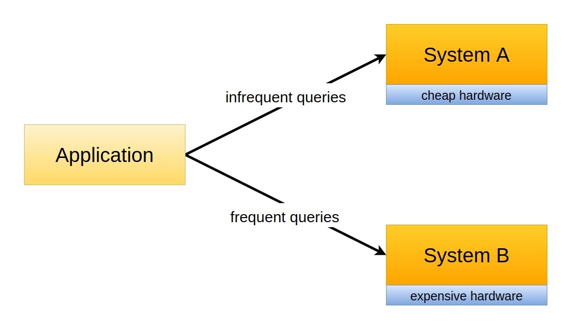
For example, we might observe that in a given social media application there are two types of queries: some are very infrequent and involve tables related to personal data and the user profile, others are extremely frequent and pretty intensive, and are related to the content shared by the user. In this case, we might decide to store the tables related to the profile and the tables that are related to content in two different systems, A and B (here, the word system might be freely replaced by computer, database, storage system, or other similar components).
This means that the infrequent queries that fetch personal data will be served by system A, while the more frequent and intensive queries related to content will be served by system B.
Suddenly, we have the chance to deploy system B using more powerful and expensive hardware, or an architecture with better performances, without increasing the cost for tables that won't benefit from such an improvement as the ones stored in system A.
This is a standard approach in system design, and it requires the introduction of an additional layer of control that will route requests to the right source. This layer might be implemented in several places, for example:
- in the code of our application, with conditional structures that query different data sources
- in the framework that we are using for the application, for example in a middleware that automatically routes requests according to nature or the query
- in a wrapper around the storage that hides the fact that data exists in two different systems
In the last case, this technique is usually called partitioning.
In this post, I will try to show the challenges we face when we partition data and focus on some of the algorithms that can be used to implement it, in particular on consistent hashing. Please note that, while some of these techniques are used by databases to provide internal partitioning, they have a wider range of applications and might come in handy in different contexts.
Design choices
Every design choice in a system depends on the requirements, and when it comes to data storage the most important factors are the nature of the data, its distribution, and the access patterns. Consider for example databases and Content Delivery Networks (CDNs): both are meant to store data, and the storage size of both can vary substantially. However, there are important differences between the two that greatly affect the design choices. Let's see some simple examples:
- databases are meant to store data in a long-term fashion, while caches are by definition short-lived. This means that an important requirement for databases is data preservation, and we should do everything in our power to avoid losing parts of the database. A cache, conversely, holds data for a short time, either predetermined by the system or forced by a change in the data source. As you can see in this case we not only take data loss as part of the equation, but we get to the point where we trigger it on purpose.
- applications often make use of range queries, which means that they retrieve sets of results spanning a range of values of one of the keys; for example, you might want to see all employers within a certain range of salaries, or all users that have more than a certain amount of followers. In such cases, it makes little sense to scatter data among different physical sources, thus making the retrieval more complicated and ultimately affecting performances. Databases see very often an access pattern of this type, while caches, being usually implemented as key/value stores, do not need to take this into account.
A practical example of partitioning
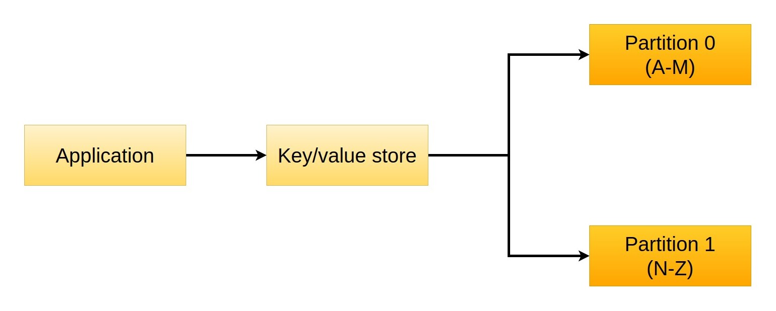
Let us consider a simple key/value store, for example a common address book where the key is the name of the contact and the value a rich document with their personal details. If multiple users access the store, chances are that the system will at a certain point struggle to serve all the requests, so we might want to partition the data to allow concurrent access. We can for example sort them alphabetically and split them in two, storing all values with a key that begins with the letters A-M in one server and the rest (keys N-Z) in the second one.
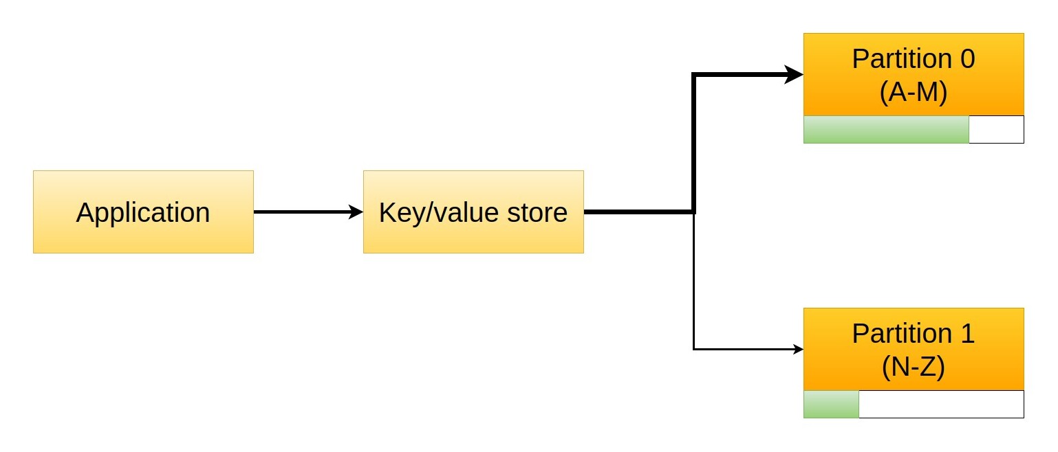
This might seem a good idea, but we will soon discover that performances are not great. Unfortunately, our address book doesn't contain the same number of people for each letter, as (for example) we know more people whose name starts with A or C than with X or Z.
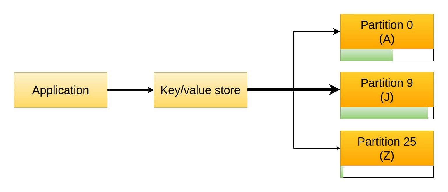
That poses a problem, as our partitioning doesn't achieve the desired outcome, that of splitting requests evenly between the two servers. If we increase the number of partitions, serving smaller groups of letters, we will just worsen the problem, to the point where a partition might be completely empty and thus receive no traffic: since the problem comes from the data distribution, we need to find a way to change that property.
One way to deal with the problem is to change the boundaries of the partitions so that we get an almost even distribution of values among them. For example, we might store keys starting with A-B in the first partition, keys starting with C-D in the second, and all the rest in the third one.
The problem with such a strategy is that it is highly dependent on the actual data that we are storing. Not only does this mean the solution has to be customised for each use case (the partitions in the example might be good for one address book and completely wrong for another), but adding data to the storage might change the distribution and invalidate the solution.
Hash functions to the rescue
An interesting solution to the problem of distributing data evenly is represented by hash functions. As I explained in my post Introduction to hashing, good hash functions produce a highly uniform distribution, which makes them ideal in this case. Please note that hash functions can help with routing queries and not with storing data. Hashed values cannot replace the content, as they are not bijective, i.e. given two different inputs the output might be the same (collision), so they can only be used to decide where to store a piece of information.
We can at this point devise a storage strategy based on hash functions. We can divide the output space of the hash function (codomain) into a certain amount of partitions and be sure that each one of them will contain a similar amount of elements. For example, the hash function might output a 32-bit number, so we know that each hashed value will be between 0 and 232 (4,294,967,295), and from here it's pretty straightforward to find partition boundaries. For example, we can create 16 partitions numbered 0 to 15, each one containing 228 hash values (268,435,456).
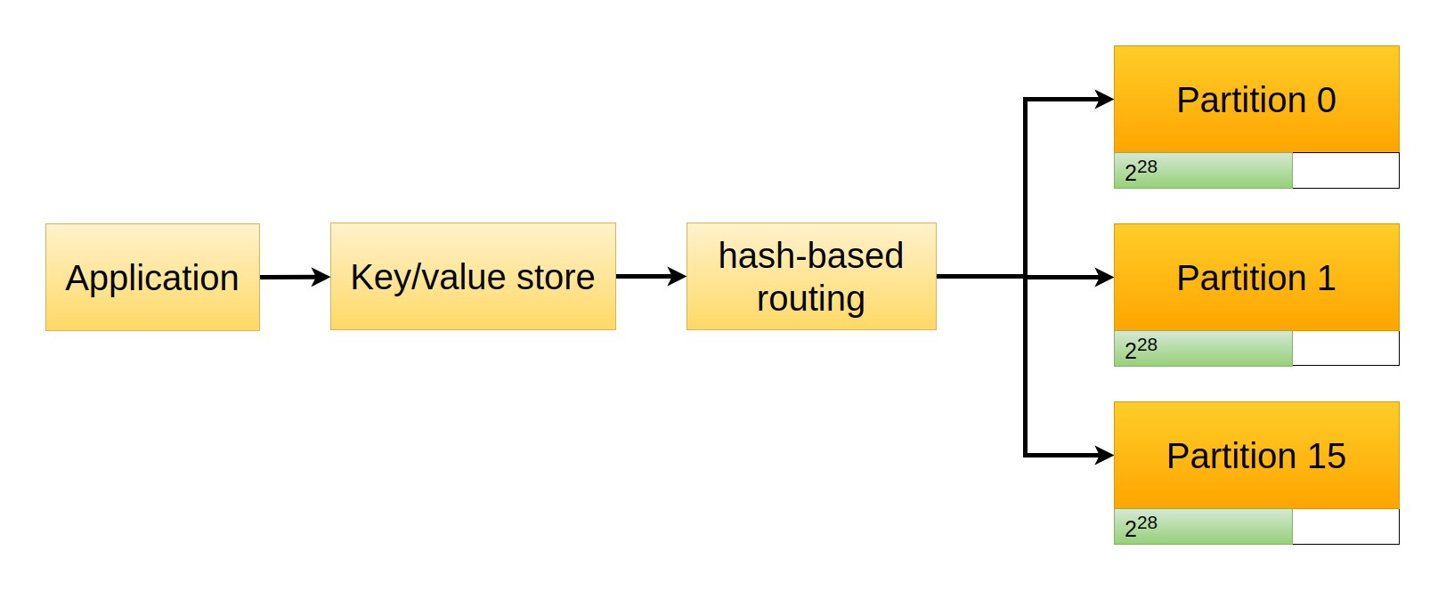
Routing is at this point very simple, as we can mathematically find the partition number given the hash. There are many ways to do this but two simple approaches are
- using the integer division
hash(k) // partition_size, e.g.hash(k) // 2**28. All keys from0to268435455end up in partition 0 (268435455 // 2**28), keys from268435456to536870911end up in partition 1, and so on.
- using the modulo operator
hash(k) % number_of_partitions, e.g.hash(k) % 16. This assigns values to partitions in a round robin fashion, where key0goes to partition 0 (0%16), key1to partition 1 (1%16), key15to partition 15 (15%16), and then starts again with key16which goes to partition 0 (16%16), and so on.
This architecture has the clear advantage that thanks to the properties of hash functions, data is scattered evenly among the partitions. This means that when we query the system, requests will also be divided evenly, thus giving us a good distribution of the load.
As we will see later, however, this is not a good approach for dynamic systems.
Partitioning use cases
Hash functions are definitely interesting but they are not the perfect solution in every case. Let's have a brief look at three different types of systems that might benefit from partitioning and discuss their specific requirements.
Load balancers
Pure load balancers solve a simple problem: to spread requests evenly across multiple identical servers. The key word here is "identical", as you cannot pick the wrong server, thus no routing can result in an error. However, spreading the load unevenly can result in performance loss, and possibly also service failure. For example, if a server gets overloaded queries might hit a timeout while waiting to be served.
For this reason, when load balancing is not content-aware, for example in a simple HTTP server scenario, round-robin partitioning is a good choice. The system just assigns new requests to servers on a rotation basis, which ensures perfectly even distribution. For example, this algorithm is the default choice for AWS Application Load Balancers.
Clearly, load balancers can be more complicated and feature-rich even without becoming content aware. The aforementioned AWS ALBs, for example, support also the "least outstanding requests" algorithm, which in simple words means choosing the server with the smallest workload.
Caches
Caches are systems that temporarily store data whose retrieval is expensive, either for the user or for the provider. For example, if a system runs a long query on a database caching the result will be beneficial both for the system and the database. For the former, because a repeated run will get the result much faster and for the latter because the load of the new query is zero.
Caches can be found everywhere and vary dramatically in size, but they are one of the best examples of systems that benefit from partitioning. As I mentioned before, their standard usage patterns don't include range queries and data loss (flushing) is part of their normal workflow.
A Content Delivery Network (CDN) is a specific type of cache that is distributed geographically. The purpose of the CDN nodes is to store content in a location that is physically near the users, thus increasing the performance of the system. This means that two geographically distinct nodes of a CDN contain the same values (replication), and the routing policy is solely based on the physical position of the user with respect to the node. Internally, each CDN node can be implemented using partitioning, though, which might speed up the performances of that specific node.
Databases
As for databases, I already mentioned that the most important problem is range queries or if you prefer, content-aware partitioning. In general, you can't partition a database without taking into account the content, or you will incur severe performance losses. So, when it comes to databases, partitioning has to be the result of a specific design and can't be applied regardless of the database schema.
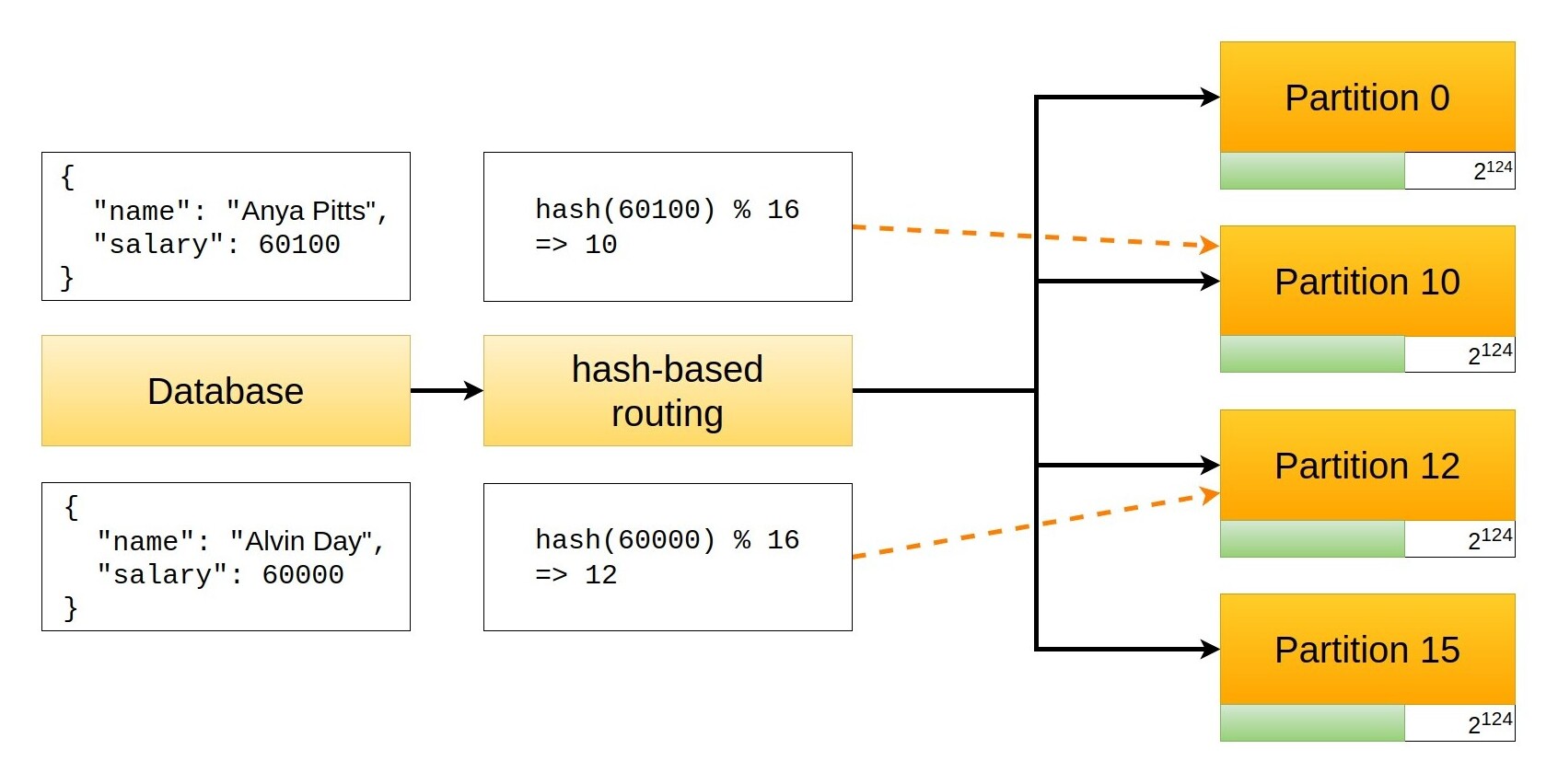
To better understand the challenge, let's consider a simple database whose elements are employees with a name and a salary. Now, if we want to partition this database we have to choose a key for the partitioning itself. It might be the primary key, the name, or the salary, as these are the only values available in each record.
Say we use hash functions to partition the database and use the employee salary as a key. Because of the properties of hash functions, employees with the exact same salary will end up being stored in the same partition, but employees with similar salaries might end up in different ones. This depends on the number of partitions, clearly, but the main point is that records that are "near" (according to the selected key) now are potentially very far.
In the example above I used MD5 as the routing hash function, and you can reproduce the calculations using the following Python code
import hashlib

def hash_value(value):
    return int(hashlib.md5(str(value).encode("utf-8")).hexdigest(), 16)

# 57500283691658467528082923406379043196
hash_value(60000)

# 209589555716047624083879134729984902154
hash_value(60100)

# 12
hash_value(60000) % 16

# 10
hash_value(60100) % 16
Things do not go much better if we use the integer division. If we have 16 partitions, each one of them contains 2124 values
# 2
hash_value(60000) // 2**124

# 9
hash_value(60100) // 2**124
Now, let's consider a query that selects all employees within a certain range of salaries. If the database is not partitioned, all records are kept on the same server, and if we optimised the system for such a query, the records will also be physically adjacent (e.g. stored in nearby memory addresses). This makes the query blazing fast, but if the database is partitioned the query has to collect values from multiple partitions which greatly penalises performance.
We can see a real example of this design challenge in the documentation of MongoDB, a non-relational database that supports partitioning (called sharding). MongoDB supports hashed sharding and ranged sharding. In their words
Hashed sharding uses either a single field hashed index or a compound hashed index as the shard key to partition data across your sharded cluster.
Range-based sharding involves dividing data into contiguous ranges determined by the shard key values. In this model, documents with "close" shard key values are likely to be in the same chunk or shard. This allows for efficient queries where reads target documents within a contiguous range. However, both read and write performance may decrease with poor shard key selection.
I highly recommend reading the two pages I linked above as they will give you a good idea of how a real system uses the concepts I introduced and what design challenges are involved when using partitioning.
Caching and scaling strategies
When we design distributed caches, an interesting problem we might face is that of scaling the system in and out to match the current load without wasting resources.
When the cache is under a light load we might want to run a small number of servers, but as soon as the number of requests increases we need to proportionally increase the number of cache nodes if we want to avoid a performance drop. This is usually not a big problem for partitioned databases, since in that case we change the number of partitions only occasionally to adjust performances or to increase the storage size, but caches like CDNs might need continuous adjustments during a single day.
Increasing or decreasing the number of nodes in a distributed cache might however be a pretty destructive action. Depending on the routing algorithm, if we add nodes (scale out) we might need to move data from existing ones to the newly added ones, and if we remove nodes (scale in) we will certainly lose the data contained in them. Both scenarios result in a (potentially massive) cache invalidation which can't be taken lightly.
The hash-based routing method presented in the previous section has terrible performances when it comes to scaling because any change in the number of servers impacts the key boundaries of the existing ones. Let's see a practical example of that and calculate the actual figures.
Scaling out with hash partitioning
Every time you consider a process or an algorithm you should have a look at how it behaves in the worst possible condition, to have a glimpse of what you might run into when you use it. For this reason, the following example considers a scale-out scenario in which all cache nodes are full. The best case is obviously when all nodes are empty, but in that case we don't need to scale out at all.
Let's consider a 32-bit hash function and 16 partitions numbered 0 to 15. Since the hash function space is 232 (4,294,967,296), each partition will contain 228 hash values (268,435,456). Each node is full, which means that all the possible 228 slots are assigned to a cached item, that is some data stored in the server that corresponds to that partition. The system is using the integer division routing system.
If we scale out to 17 partitions, increasing the pool by just by 1 node, each node will now contain a smaller part of the global data space, as now we split it among more nodes. In particular, each node used to contain 1/16 of the global data (268,435,456), and will now contain 1/17 of it (approx. 252,645,135). Our biggest problem is now managing the transition between the initial setup and the new one.
The first node hosted 1/16 of the data space, the keys from 0 to 268435455. It will now contain 1/17 of the data space, the keys from 0 to 252645134. To simplify the example it is useful to convert everything into a common unit of measure: the node used to contain 17/272 of the space (1/16) and contains now 16/272 (1/17) of it.
This means that 1/272 of the whole data space has to be moved to the second node, corresponding to the keys from 252645135 to 268435455. It is important to note that these keys cannot be moved to the newly added node, but have to be moved to the second node because the algorithm we use maps keys to nodes in order.
This means that the second node will receive 1/272 of the whole data space. Since it originally already contained 17/272 of the whole space it should now theoretically contain 18/272 of it. However, as it happened for the first node, we want to balance the content and reduce it to 16/272, so now we have 2/272 of the whole space that we want to move to the third node.
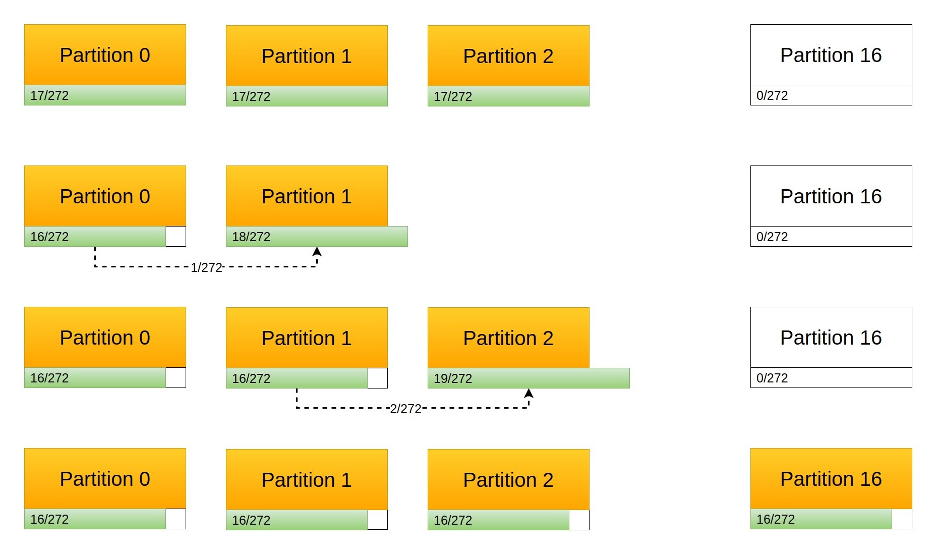
So, we move 1/272 from node 1 to node 2, 2/272 from node 2 to node 3, 3/272 from node 3 to node 4, and going on with the example we end up moving 16/272 (1/17) from the 16th node to the 17th, which fills it with the correct amount of keys. However, in doing so we moved 136/272 (1/272 + 2/272 + 3/272 + ... + 16/272) of the data space between nodes, which is exactly 50% of it.
So, for any initial size and a scale out of 1 single node, we have to move 50 of the data stored in our cache, and it might only get worse by increasing the number of final nodes until we end up having to move almost 100 of it (in an extreme case). A similar effect plagues the scale-in action, where one or more nodes are removed from the pool, and the keys they contain have to be migrated to the remaining nodes, creating a ripple effect to redistribute the keys according to the algorithm.
Using a modulo routing strategy doesn't change things: as I mentioned before, the core issue is that the addition of new nodes changes the routing of the whole data space, requiring a massive migration of keys in the entire system.
A different approach
While the idea of using hash functions looked very promising, we quickly found that the trivial implementation has very poor performances in a dynamic setting. As we clearly saw in the previous section, the problem is that upon scaling more than half of the keys have to be moved across nodes, so if we could find a way to avoid this we could still use hash functions to scatter data uniformly across the nodes.
As you might have already figured out, the issue comes from the attempt to keep all nodes perfectly balanced. The modulo and integer division algorithms distribute keys evenly (as long as the hash function has a good diffusion), but this is a double-edged sword. The balance is extremely beneficial in a static environment, but it is also the Achilles heel of this architecture when we change the number of nodes.
When we design a system, requirements are paramount. Everything we add to the final product should be there to satisfy one or more requirements. However, often requirements clash with each other, and trying to implement all of them at once might lead to situations where there is no apparent solution. In such cases, it is useful to temporarily drop one or more requirements and investigate the options we have, and this is exactly what we can do in this case: maintaining balance is an important feature, but let's see what would happen if we didn't have that requirement.
If we don't care about balancing nodes we can solve the problem with a different approach. Instead of using the integer division to find the slot, we can keep a table of the minimum hash served by each slot and route requests according to that. Each row of the table will have a minimum hash and the node that serves them.
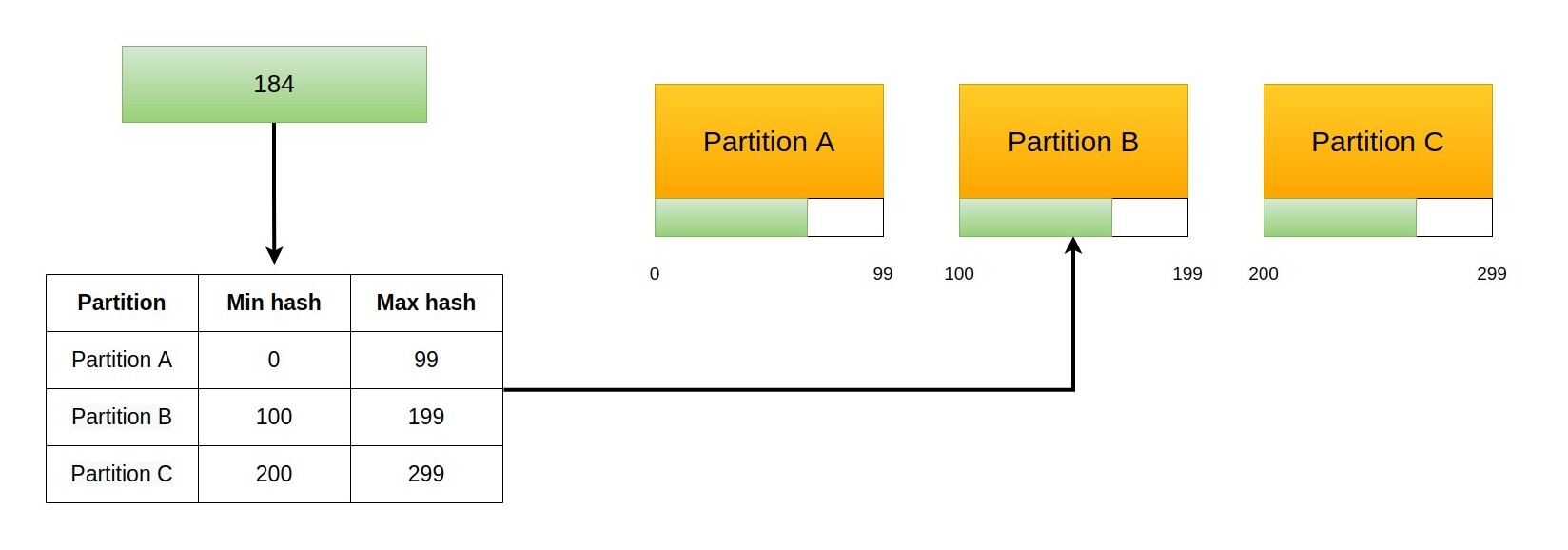
This means that when we increase the number of slots we can just drop a new slot anywhere and assign to it all the keys that fall under its domain. This means that the new node will become the owner of keys that belonged to another node as it happened before, but with an important difference. Now all keys come from another single node, and the amount of keys moved is a fraction of those contained in it (which is much less than half of the keys). In the worst case, we need to move all keys contained in a node, which once again is much less than half of the keys.
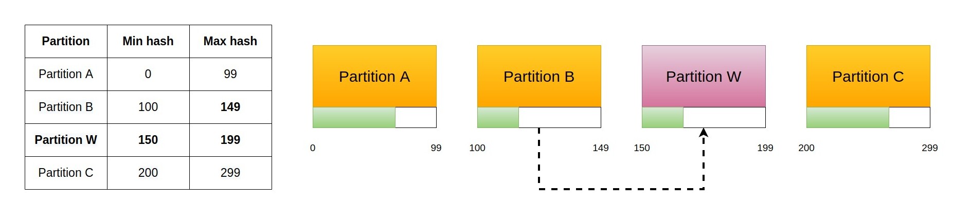
As you can see, this relieves the load of one single node. According to what we said before, we are not trying to balance the load of the whole cluster. If we could use this technique to cover multiple spaces with a single added node, though, we could relieve the load of more than one other node. In principle this is simple: we just need to add multiple rows with the same node to the table.
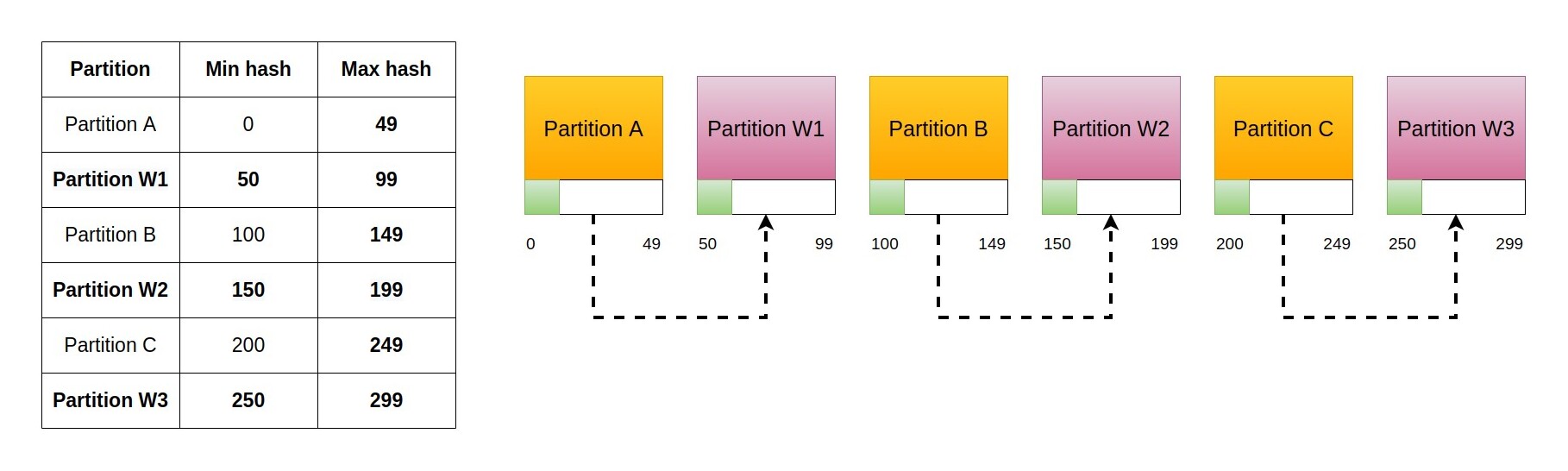
Pay attention to the fact that we added multiple rows, that is multiple partitions, but they are all served by the same physical node. This has several advantages:
- It fills the new node with keys coming from several different nodes without rippling effects.
- The key transfer load is spread among different nodes, noticeably hitting only the new node.
There is also an interesting turn of events: since keys for the new node are fetched from several different existing nodes, the process will keep the cluster balanced! This is a remarkable outcome: we temporarily dropped a requirement and found a solution that provides that exact requirement in a different way.
The key part of this new process is the idea that multiple partitions can be served by the same node. The only missing part at this point is a way to identify the new partitions (the sets of hashes) served by the new node in a deterministic way.
Consistent hashing
Finally, let me introduce consistent hashing as a technique to implement the process described above.
As we discussed in the previous section, the only missing part is an algorithm that produces a deterministic set of hash ranges for a single new node. These hash ranges represent the partitions served by that node and should be scattered across the whole hash space. It is important for them to be spread because this way they will each receive some keys from existing nodes, instead of migrating a bulk of keys from a single one. The more evenly spread, the better the distribution of the load and the more balanced the resulting cluster.
As we saw previously, any time we need to scatter data across a given space in a deterministic way, hash functions are a good choice, and they can be used in this case as well. The idea is simple: each partition of a node is assigned a name and this name is hashed with the same function used to hash the keys stored in the system. This will produce a deterministic value in the hash space, and that value will be the minimum value served by that partition. Thanks to diffusion the names of all partitions will generate different hash values that won't easily clash, and this is the way we generate the routing table.
Let's see an example, bearing in mind that the specific function can change among implementations.
For simplicity's sake, I used a custom hash function that outputs 28-bit hashes (7 hexadecimal digits). This makes it possible to compare hashes visually and simplifies the example. To do this I took the first 7 digits of the SHA1 hash with the following Python code
def hash_name(name):
    return int(hashlib.sha1(name.encode("utf-8")).hexdigest()[:7], 16)
thus creating a hash function whose values go from 0x0000000 to 0xfffffff. At the end of the post you will find the Python code that I used to generate the following routing tables, and you are free to experiment using different settings.
WARNING: this is not a good hash function! SHA1 produces 160 bits hashes, so taking the first 28 bits reduces the hash space to a microscopic fraction of the total, as we go from 2160 total hashes to 228. Please keep in mind that this is done only to simplify the visualisation of the example.
All our nodes are called server-X with X being a letter of the English alphabet, thus giving us server-a, server-b, and so on. I decided to create 5 partitions per server, numbered from 0 to 4, which are generated appending -Y to the name, where Y is the number of the partition. For example:
server-a-0 -- hash --> 148456820
server-a-1 -- hash --> 57674441
server-a-2 -- hash --> 216250418
server-a-3 -- hash --> 30595746
server-a-4 -- hash --> 23746828
If we do this for two nodes (server-a and server-b) and then sort the results we will get a full routing table
 23746828 --> server-a-4 ( 6848918 hashes)
 30595746 --> server-a-3 (27078695 hashes)
 57674441 --> server-a-1 ( 3228787 hashes)
 60903228 --> server-b-2 (17957108 hashes)
 78860336 --> server-b-0 ( 7773725 hashes)
 86634061 --> server-b-4 (61822759 hashes)
148456820 --> server-a-0 (67793598 hashes)
216250418 --> server-a-2 (17304439 hashes)
233554857 --> server-b-3 (29289666 hashes)
262844523 --> server-b-1 ( 5590932 hashes)
Remember that the hashes in the routing table are the minimum hash served by that partition. For example, the first line tells us that all hashes from 23746828 are served by the partition server-a-4, while hashes from 30595746 are served by the partition server-a-3. This means that the partition server-a-4 serves 6848918 hashes (as you can read in the table). A key whose hash is 79249022 will be served by server-b-0
 60903228 --> server-b-2 (17957108 hashes)
 78860336 --> server-b-0 ( 7773725 hashes)
                     ^
                     |
 79249022 -----------+

 86634061 --> server-b-4 (61822759 hashes)
148456820 --> server-a-0 (67793598 hashes)
Since partitions are not physically separated, but are just virtual entities belonging to a node, the route table can be simplified to
 23746828 -- > server-a (37156400 hashes)
 60903228 -- > server-b (87553592 hashes)
148456820 -- > server-a (85098037 hashes)
233554857 -- > server-b (34880598 hashes)
What we achieved is remarkable, but there are still two problems. Let's have a look at a simple routing table for three nodes with 5 partitions each
 23746828 --> server-a (23267855 hashes)
 47014683 --> server-c (10659758 hashes)
 57674441 --> server-a ( 3228787 hashes)
 60903228 --> server-b (63557309 hashes)
124460537 --> server-c (23996283 hashes)
148456820 --> server-a (31382512 hashes)
179839332 --> server-c (36411086 hashes)
216250418 --> server-a (17304439 hashes)
233554857 --> server-b (15386579 hashes)
248941436 --> server-c (13903087 hashes)
262844523 --> server-b ( 5590932 hashes)
First, the lowest value is not 0, which means that there are some hashes (23,746,828 in this case) which are not served by any slot. Second, in general the distribution doesn't cover the space evenly, as some nodes receive too many keys compared to others. This second problem isn't actually visible in the setups I showed so far, but it becomes noticeable increasing the number of servers. For example, with two nodes we have this situation
server-a: 122254437 hashes
server-b: 146181018 hashes
while with 5 nodes it becomes
server-a: 64211359 hashes
server-b: 66179053 hashes
server-c: 57545779 hashes
server-d: 43217324 hashes
server-e: 37281940 hashes
As you can see, in the second case the load of server-e is 56% that of server-b.
The first problem is easily solved assigning the initial hashes to the last node, that is considering the hash space mapped on a circle. This means that for 2 nodes with 5 partitions each we have
Full routing table
        0 --> server-b-1 (23746828 hashes)
 23746828 --> server-a-4 (6848918 hashes)
 30595746 --> server-a-3 (27078695 hashes)
 57674441 --> server-a-1 (3228787 hashes)
 60903228 --> server-b-2 (17957108 hashes)
 78860336 --> server-b-0 (7773725 hashes)
 86634061 --> server-b-4 (61822759 hashes)
148456820 --> server-a-0 (67793598 hashes)
216250418 --> server-a-2 (17304439 hashes)
233554857 --> server-b-3 (29289666 hashes)
262844523 --> server-b-1 (5590932 hashes)

Simplified routing table
        0 -- > server-b (23746828 hashes)
 23746828 -- > server-a (37156400 hashes)
 60903228 -- > server-b (87553592 hashes)
148456820 -- > server-a (85098037 hashes)
233554857 -- > server-b (34880598 hashes)
where the partition server-b-1 contains the orphaned initial hashes.
The second problem is a matter of statistical approach. The hash function that we use to map the partition name to the key space cannot be controlled, as its diffusion property has been designed to avoid a regular spacing of values. However, if we increase the number of partitions we expect the hash function to spread values across the whole space. At that point, each partition will be assigned just a tiny key space, and the differences between partitions will be less noticeable. In other words, by increasing the number of partitions dramatically we should achieve a better distribution. Let's compare the results of 5 nodes with 2 partitions each
server-a 36500586
server-b 76678431
server-c 31738329
server-d 56183426
server-e 67334683
with the results of 5 nodes with 3000 partitions each
server-a 53385222
server-b 53855877
server-c 53755762
server-d 53597662
server-e 53840932
There is clearly an upper limit to the number of partitions that we can create. If we create more partitions than the possible number of hashes we will end up having empty ones and incurring routing errors as some of them will clash, but this is a purely theoretical case: using standard real hash functions we generate hashes of at least 160 bits, which means a codomain of 2160 possible values (more than 1048). With 10,000 nodes (which is a considerable amount of servers in 2022) the threshold would be greater than 1044 partitions per server.
So far, we achieved great results, but we already managed to properly partition the space with simple techniques. The real power of consistent hashing is in the way it behaves in a dynamic setting.
Consistent hashing and scaling
The interesting thing about consistent hashing is its amazing behaviour in a dynamic environment. As you might remember, the problem with hash partitioning was that a change in the number of nodes had ripple effects that resulted in a massive migration of at least half the keys.
With consistent hashing, when we add a new node we need to generate the hash values for that and put them in the routing table, and at that point we need to migrate the keys that fall under the domain of the newly created slots. Let's see an example before we discuss the performances.
The initial setup is 2 nodes with 5 partitions each
Full routing table
        0 --> server-b-1 (23746828 hashes)
 23746828 --> server-a-4 (6848918 hashes)
 30595746 --> server-a-3 (27078695 hashes)
 57674441 --> server-a-1 (3228787 hashes)
 60903228 --> server-b-2 (17957108 hashes)
 78860336 --> server-b-0 (7773725 hashes)
 86634061 --> server-b-4 (61822759 hashes)
148456820 --> server-a-0 (67793598 hashes)
216250418 --> server-a-2 (17304439 hashes)
233554857 --> server-b-3 (29289666 hashes)
262844523 --> server-b-1 (5590932 hashes)

Simplified routing table
        0 -- > server-b (23746828 hashes)
 23746828 -- > server-a (37156400 hashes)
 60903228 -- > server-b (87553592 hashes)
148456820 -- > server-a (85098037 hashes)
233554857 -- > server-b (34880598 hashes)

Stats
server-a 122254437
server-b 146181018

TOTAL HASHES: 268435455/268435455
if we add one node we migrate to this new setup
Full routing table
        0 --> server-b-1 (23746828 hashes)
 23746828 --> server-a-4 (6848918 hashes)
 30595746 --> server-a-3 (16418937 hashes)
 47014683 --> server-c-3 (10659758 hashes)
 57674441 --> server-a-1 (3228787 hashes)
 60903228 --> server-b-2 (17957108 hashes)
 78860336 --> server-b-0 (7773725 hashes)
 86634061 --> server-b-4 (37826476 hashes)
124460537 --> server-c-2 (23996283 hashes)
148456820 --> server-a-0 (31382512 hashes)
179839332 --> server-c-1 (25303093 hashes)
205142425 --> server-c-4 (11107993 hashes)
216250418 --> server-a-2 (17304439 hashes)
233554857 --> server-b-3 (15386579 hashes)
248941436 --> server-c-0 (13903087 hashes)
262844523 --> server-b-1 (5590932 hashes)

Simplified routing table
        0 -- > server-b (23746828 hashes)
 23746828 -- > server-a (23267855 hashes)
 47014683 -- > server-c (10659758 hashes)
 57674441 -- > server-a ( 3228787 hashes)
 60903228 -- > server-b (63557309 hashes)
124460537 -- > server-c (23996283 hashes)
148456820 -- > server-a (31382512 hashes)
179839332 -- > server-c (36411086 hashes)
216250418 -- > server-a (17304439 hashes)
233554857 -- > server-b (15386579 hashes)
248941436 -- > server-c (13903087 hashes)
262844523 -- > server-b ( 5590932 hashes)

Stats
server-a 75183593
server-b 108281648
server-c 84970214

TOTAL HASHES: 268435455/268435455
Let's have a closer look to what happens with server-c
Simplified routing table
        0 -- > server-b (23746828 hashes)
 23746828 -- > server-a (23267855 hashes) ----+ 10659758 hashes
                                              | from server-a
 47014683 -- > server-c (10659758 hashes) <---+
 57674441 -- > server-a ( 3228787 hashes)
 60903228 -- > server-b (63557309 hashes) ----+ 23996283 hashes
                                              | from server-b
124460537 -- > server-c (23996283 hashes) <---+
148456820 -- > server-a (31382512 hashes) ----+ 36411086 hashes
                                              | from server-a
179839332 -- > server-c (36411086 hashes) <---+
216250418 -- > server-a (17304439 hashes)
233554857 -- > server-b (15386579 hashes) ----+ 13903087 hashes
                                              | from server-b
248941436 -- > server-c (13903087 hashes) <---+
262844523 -- > server-b ( 5590932 hashes)
Globally, server-c receives 47,070,844 hashes from server-a and 37,899,370 hashes from server-b, which results in a migration of approximately 30% of the total hashes. As you can see there is no ripple effect here, as the boundaries of the existing partitions do not change.
Let's consider the performances in the worst case when we add one single node. If we are terribly unlucky (and we use a hash function with clear issues) each partition of the new node will cover completely a partition of an existing node. Assuming that the initial setup with N nodes created a balanced cluster, each node contains 1/Nth of the total keys, and in the worst case we need to move all of them from an existing node to the newly added one.
So, adding one node to a cluster of N nodes using consistent hashing results, in the worst case, in the migration of 1/Nth of the keys. In the previous example, then, we expected to migrate at most 50% of the keys (1/2), and we ended up migrating 30$ of them.
This is a terrific result. Not only it's much better than the previous one (at least 50% of the keys), but it gets better increasing the size of the cluster. In a cluster with 100 nodes, adding a node will result (in the worst case!) in the migration of 1/100 of the keys.
Source code
All routing tables shown in the post have been created with the following Python script. Please bear in mind that this is just demo code, so things haven't been optimised or designed particularly well. Feel free to change the hash function and the parameters of the script to experiment and see what consistent hashing can do.
consistent_hashing_demo.pyimport hashlib
import itertools
import sys
import string
from operator import itemgetter
NUM_NODES = 3
NUM_PARTITIONS = 5
def hash_name(name):
encoded_name = name.encode("utf-8")
hash_encoded_name = hashlib.sha1(encoded_name).hexdigest()
return int(hash_encoded_name[:7], 16)
def create_partitions(node_name, partitions):
partition_hashes = []
for partition_number in range(partitions):
partition_name = f"{node_name}-{partition_number}"
partition_hash = hash_name(partition_name)
partition_hashes.append(
{
"min_hash": partition_hash,
"partition_name": partition_name,
"node_name": node_name,
}
)
return partition_hashes
def create_routing_table(node_names, partitions):
table = []
for node_name in node_names:
table.extend(create_partitions(node_name, partitions))
table = sorted(table, key=itemgetter("min_hash"))
return table
if NUM_NODES > len(string.ascii_lowercase):
print("Too many servers")
sys.exit(1)
nodes = [f"server-{i}" for i in string.ascii_lowercase[:NUM_NODES]]
routing_table = create_routing_table(nodes, NUM_PARTITIONS)
routing_table = [
{
"min_hash": 0,
"partition_name": routing_table[-1]["partition_name"],
"node_name": routing_table[-1]["node_name"],
}
] + routing_table
routing_table_shift = routing_table[1:] + [
{"min_hash": 0xFFFFFFF, "partition_name": "END"}
]
full_routing_table = []
for i, j in zip(routing_table, routing_table_shift):
full_routing_table.append(
{
"min_hash": i["min_hash"],
"partition_name": i["partition_name"],
"node_name": i["node_name"],
"served_hashes": j["min_hash"] - i["min_hash"],
}
)
print("Full routing table")
for r in full_routing_table:
print(f'{r["min_hash"]:9} --> {r["partition_name"]} ({r["served_hashes"]} hashes)')
grouped_routing_table = itertools.groupby(
full_routing_table, key=itemgetter("node_name")
)
simplified_routing_table = []
for r in grouped_routing_table:
consecutive_partitions = list(r[1])
simplified_routing_table.append(
{
"node_name": r[0],
"min_hash": consecutive_partitions[0]["min_hash"],
"served_hashes": sum([i["served_hashes"] for i in consecutive_partitions]),
}
)
print()
print("Simplified routing table")
for r in simplified_routing_table:
print(f'{r["min_hash"]:9} -- > {r["node_name"]} ({r["served_hashes"]:8} hashes)')
print()
print("Stats")
stats = []
for node in nodes:
slots = filter(lambda x: x["node_name"] == node, simplified_routing_table)
total_hashes = sum([i["served_hashes"] for i in slots])
stats.append({"node_name": node, "served_hashes": total_hashes})
for r in stats:
print(r["node_name"], r["served_hashes"])
total_hashes = sum([i["served_hashes"] for i in stats])
print()
print(f"TOTAL HASHES: {total_hashes}/{2**28 - 1}")
Final words
I hope this long post was useful to introduce you to the topic of partitioning and in general to system design. As I mentioned, such concepts are currently in use by well-known systems, and still discussed as none of them is perfect, so it is worth understanding the fundamental issues before adopting a specific solution.
Resources
- Martin Kleppmann, Designing Data-Intensive Applications, Chapter 6 "Partitioning", O’Reilly 2017 official site.
- The Wikipedia article about consistent hashing.
- A Guide to Consistent Hashing by Juan Pablo Carzolio.
- The original article by David Karger et al.: "Consistent Hashing and Random Trees: Distributed Caching protocols for Relieving Hot Spots ont the World Wide Web".
- An alternative algorithm by John Lamping and Eric Veach: "A Fast, Minimal Memory, Consistent Hash Algorithm".
Feedback
Feel free to reach me on Twitter if you have questions. The GitHub issues page is the best place to submit corrections.
Related Posts


Public key cryptography: RSA keys
Updated on

Dissecting a Web stack
Updated on


Clean Architectures in Python: the book
Updated on


From Docker CLI to Docker Compose
Updated on